Making a Memory Element for Quantum Computers

In my first blog post, I want to talk about a paper that my co-authors and I wrote back in 2024 about making a memory element for quantum computers.

Quantum computers promise to solve certain computational problems exponentially faster than even today’s most powerful supercomputers. The quintessential example is Shor’s Algorithm [1], which proves that quantum computers can factor integers in polynomial time. There is no known efficient classical algorithm for achieving this task, a fact that underpins much of today’s encryption, such as RSA.

It turns out there are many architectures for building a quantum computer. Some prominent examples include:

• Trapped ions: This architecture involves encoding information in the energy levels of an ion (typically an atom with a charge due to one missing electron). Companies working on this technology include IonQ, Quantinuum, and Alpine Quantum Technologies.
• Neutral atoms: This architecture involves encoding information in the energy levels of neutral atoms (i.e., atoms with no net charge) held in optical tweezers. Companies working on this technology include QuEra, Pasqal, Atom Computing, and Infleqtion.
• Photonics: This architecture relies on using particles of light (photons). Approaches often involve preparing a unique quantum state, known as a cluster state, and using clever measurements to execute computation. Companies working on this technology include PsiQuantum, Xanadu, and ORCA Computing.
• Silicon spin qubits: This architecture encodes quantum information in the spin degree of freedom of electrons confined in silicon, using either gate-defined quantum dots or defects (like phosphorus). Companies working on this technology include Intel, Silicon Quantum Computing, and Diraq.
• Superconducting qubits: This architecture encodes quantum information in the quantum states of superconducting circuits (typically utilizing Josephson junctions) that are manipulated using microwaves. Companies working on this technology include IBM, Google Quantum AI, AWS, Rigetti, and IQM.

I’m particularly interested in superconducting qubits, a field often referred to as circuit QED [2]. Circuit QED is a promising platform for quantum computing because it allows us to fabricate quantum bits (qubits) using standard semiconductor fabrication processes. This provides significant control over qubit design, a distinct advantage over atomic platforms where energy levels are fixed by nature. However, like all quantum platforms, Circuit QED faces major challenges regarding hardware overhead.

For instance, it is estimated that we will need between \(10^6\) and \(10^8\) physical qubits to perform fault-tolerant computations like factoring large numbers [3]. This creates a massive scaling issue: unless we develop clever multiplexing solutions, each qubit currently requires its own control line. This “wiring bottleneck” is not a scalable solution.

A Hardware-Efficient Approach

To address this, there are proposals for hardware-efficient quantum computing that rely on high-quality delay lines [4, 5, 6]. You can think of a delay line like a long string anchored to a wall. When you pluck one end, a pulse travels down the string, bounces off the anchor, and returns to you. The pulse is effectively “delayed” by the travel time. Similarly, for pulses of light, imagine an optical fiber with a mirror on one end. If you launch a light pulse into the fiber, it flies down, reflects, and returns—again, effectively delayed.

The concept of using delay lines is central to building a photonic quantum computer. By connecting a quantum emitter to a delay line, we can store quantum information within the delay itself. By carefully performing operations on the emitter when it re-interacts with the delayed pulse, we can generate an exotic resource known as a cluster state [7]. These cluster states are the fuel for fault-tolerant, measurement-based quantum computing.

The problem for superconducting qubits is that standard delay lines would need to be prohibitively long. Achieving a mere 1 microsecond delay would require a waveguide over 100 meters long. This cannot be easily fabricated on a chip. However, researchers have developed clever approaches to solve this, such as making metamaterial delay lines that effectively slow down light as it propagates on a chip [8].

A Parametrically Programmable Delay Line

In this work [9], my co-authors and I presented another approach to solving this problem. Crucially, instead of just delaying the pulse of light, our delay line lets the experimenter manipulate the light while it is in the delay line!

There are two physical concepts that I need to introduce very quickly for you to understand our work:

1. Parametric interactions: Parametric interactions allow us to move energy from one system to another despite the two systems operating at very different frequencies. In physics, frequency and energy are proportional, and because energy is conserved, two systems cannot efficiently swap energy if they are at different frequencies. For example, if system A oscillates at frequency \(\omega_a\) and system B oscillates at frequency \(\omega_b\), then they cannot efficiently swap energy unless \(\omega_a \simeq \omega_b\). Parametric interactions refer to when you supply additional energy to make up for any energy difference. For example, if we supply energy to system B at frequency \(\omega_d\) such that \(\omega_a \simeq \omega_b + \omega_d\), then systems A and B can swap energy. Crucially, parametric interactions require some form of nonlinearity to be possible.
2. Delay lines: Again, you should imagine a delay line as a long string that is anchored to a wall, or an optical fiber with a mirror at the end. When you pluck one end of the string, or when you send in a pulse of light, the excitation flies down the string/fiber until it reaches the wall/mirror, bounces back, and then comes back to you. Let’s stick with the string analogy. The string actually has many “eigenmodes” that oscillate at different frequencies.

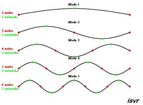Figure 1: The eigenmodes of a string. When you pluck a string, you excite a sum of the eigenmodes. If you pluck one end of the string, the dynamics looks like a pulse that propagates back and forth along the string. Taken from here.

The first eigenmode should be familiar to you from trampolines. Crucially, the eigenmode frequencies are all equally spaced by a number called the free-spectral range (FSR). When you pluck one end of the string, you excite all the eigenmodes, and the dynamics that you observe are really just the sum of all the eigenmodes. The evolution of this sum looks like a pulse flying down the string. At a time \(t=1/\text{FSR}\), your pulse has returned to where you plucked the string.

Building a “Virtual” Delay Line

In our system, we have one element (known as an Asymmetrically Threaded SQUID or ATS [10]) that enables parametric interactions. We use these parametric interactions to take a microwave pulse, which encodes the information we want to store, and swap it into 7 resonators that form the eigenmodes of a virtual delay line. I say “virtual” delay line here because, unlike a physically real delay line where the information is stored in standing waves, now the information is stored across 7 physically separate resonators. Our delay line operates at 5 GHz, which is a pretty standard frequency for superconducting qubits.

What’s cool about this system is that because we are using parametric interactions to move the pulse around, we can control the properties of the delay line while the information is being stored. For example, we can send in a pulse of light and then trap it by turning off the parametric interactions. Then we can get the pulse back out at a later time by turning the parametric interactions back on.

In the figure below, we launch a microwave pulse at the delay line at time \(t=0\) and then trap it for \(t=2, 4, 6\) microseconds. The small pulse you see at time \(t=0\) is reflected light from some impedance mismatch. 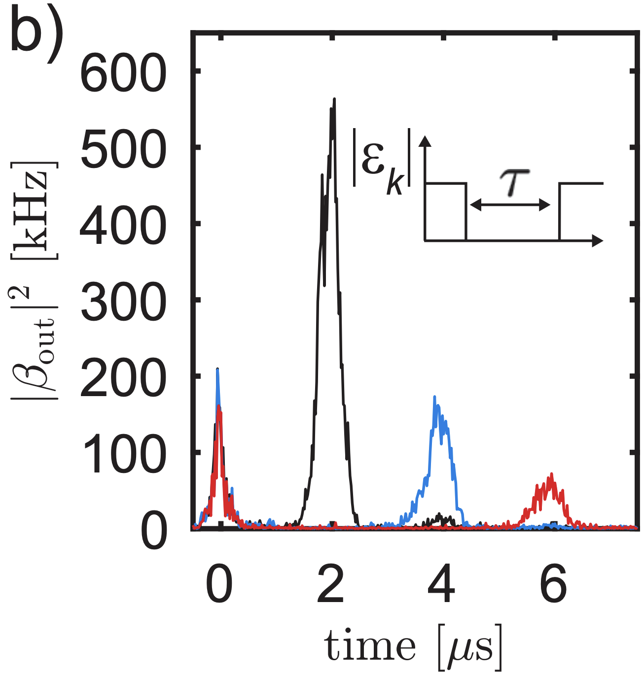Figure 2: Trapping and re-emitting a microwave pulse in a virtual delay line.

Limitations and Looking Forward

The main limitation of our chip was that our storage resonators were pretty lossy. That’s why, in the figure above, the red pulse is much smaller than the black pulse.

The long-term goal of this chip would be to connect it to a qubit and use it as a memory element for true superconducting qubit signals, unlike the classical pulses that we used in our experiment. An even cooler goal would be to actually use our chip to make a cluster state.

References

[1] Shor, P. W. (1994). “Algorithms for quantum computation: discrete logarithms and factoring.” Proceedings of the 35th Annual Symposium on Foundations of Computer Science, 124–134.
[2] Wallraff, A., et al. (2004). “Strong coupling of a single photon to a superconducting qubit using circuit quantum electrodynamics.” Nature, 431, 162–167.
[3] Fowler, A. G., et al. (2012). “Surface codes: Towards practical large-scale quantum computation.” Physical Review A, 86(3), 032324.
[4] H. Pichler, S. Choi, P. Zoller, and M. D. Lukin. (2017). “Universal photonic quantum computation via time-delayed feedback.” Proceedings of the National Academy of Sciences 114, 11362.
[5] K. Wan, S. Choi, I. H. Kim, N. Shutty, and P. Hayden. (2021). “Fault-tolerant qubit from a constant number of components.” PRX Quantum 2, 040345.
[6] Takeda, S., & Furusawa, A. (2017). “Universal quantum computing with arbitrary continuous-variable cluster states.” Physical Review Letters, 119(12), 120504.
[7] Raussendorf, R., & Briegel, H. J. (2001). “A one-way quantum computer.” Physical Review Letters, 86(22), 5188.
[8] Ferreira, Vinicius S., et al. (2024). “Deterministic generation of multidimensional photonic cluster states with a single quantum emitter.” Nature Physics 20.5: 865-870.
[9] Makihara, Takuma, et al. (2024). “A parametrically programmable delay line for microwave photons.” Nature Communications 15.1: 4640.
[10] Lescanne, Raphaël, et al. (2020). “Exponential suppression of bit-flips in a qubit encoded in an oscillator.” Nature Physics 16.5: 509-513.